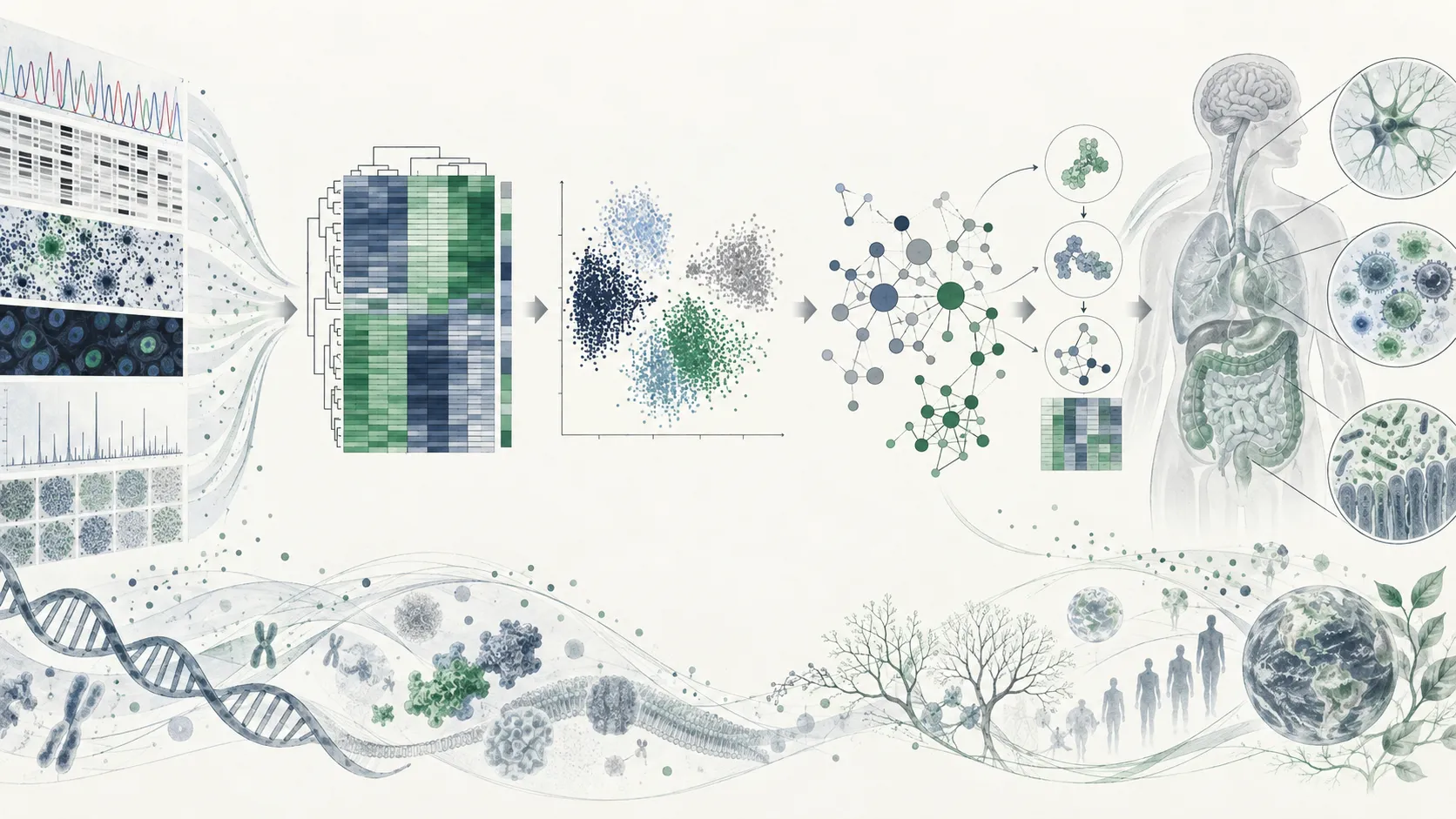
From FASTQ to insights: Practical transcriptomic pipelines & batch effect handling — Research Note

Transcriptomic pipeline: sequencing chromatogram, pseudoalignment, and expression profiling

Evolution of Transcriptomic Quantification

Early RNA-seq pipelines relied heavily on splice-aware genomic aligners (e.g. STAR, HISAT2) followed by counting tools like featureCounts. While essential for novel isoform discovery or fusion transcript identification, these approaches require massive memory footprints (32+ GB RAM) and hours of compute time per sample.

For established model organisms, k-mer pseudoalignment (Kallisto / Salmon) provides accurate transcript abundance estimation in minutes while decoupling read quantification from heavy alignment SAM/BAM generation.

Key Workflow Stages

Decoy-Aware Indexing

Building transcriptome indices with the whole genome as a decoy sequence prevents chimeric or intergenic reads from erroneously aligning to homologous transcripts.

Tximport Transcript-to-Gene Aggregation

Summarizing transcript-level estimated counts to gene-level matrices using tximport accounts for potential gene length changes across experimental conditions.

Empirical Bayes Dispersion Shrinkage

Applying DESeq2 with apeglm shrinkage stabilizes log2 fold change estimates for low-count genes without inflating false-positive rates.

Surrogate Variable Analysis (SVA)

Modeling hidden batch effects and technical confounders using SVA or ComBat-seq protects downstream statistical tests from laboratory artifact inflation.

Never rely on raw p-values when analyzing high-dimensional gene expression; strict false discovery rate (FDR) control is non-negotiable.

Downstream Biological Interpretation

Disciplined Filtering: Apply both statistical significance ( $p_{\text{adj}} < 0.05$ via Benjamini-Hochberg) and biological magnitude thresholds ( $|\log_2\text{FC}| \ge 1.0$ ) rather than reporting marginal differences.
Gene Set Enrichment (GSEA): Perform rank-based GSEA (using log2FC $\times -\log_{10}p$ as the ranking metric) against MSigDB or Reactome to detect coordinated pathway shifts without arbitrary cutoff biases.
Reproducibility Archiving: Export normalized Variance Stabilizing Transformation (VST) matrices alongside tidy metadata manifests to enable instant re-analysis in R or Python.